Bluetooth Low Energy Asset and Personnel Tracking, BLE-APT
Visit my Github for the most updated code: https://github.com/Techryptic/BLE-APT
BLE-APT develops a ‘digital fingerprint’ to identify BLE devices using MAC address randomization for security. That is, given a BLE device with a continually changing MAC address, identify digital and physical features from packet transmissions that could be used as a digital fingerprint to say this is device X.
Although BLE has security & privacy mechanisms built into the protocol, this project shows that you can fingerprint and track BLE devices. BLE devices (Fitbits, Apple Watch, ect.) are always sending out packets, even when not connected to it’s central device. Abusing this as shown below, can enable you to do positional tracking of devices.
Requirements
Ubertooth One
Ubuntu
Wireshark (Not needed, but useful)

Python 3.6+
plotly
chart-studio
dash
pandas-datareader
peakutils
fuzzywuzzy
scipy
ubertooth
Main.py ::
Main.py will be the start of the collection. It’s broken in two parts, input file or live capture.
If going the input route, you’ll run the following command:
ubertooth-btle -fI -r example.pcapng | sed -e 's|["'\'']||g' | xargs | sed -e 's/systime/\nsystime/g' >> example.txt
Essentially, ubertooth is running with the follow option and exporting to example.pcapng, that information is pipped to sed & xargs and back to sed for some cleanup and finally writing to example.txt. Example.txt would be the input file for Main.py.
python3.8 Main.py input example.txt output.csv
If going the live capture route, you’ll run the following command (same as above):
* ubertooth-btle -fI -r example.pcapng | sed -e 's|["'\'']||g' | xargs | sed -e 's/systime/\nsystime/g' >> example.txt
and within another terminal you’ll run the follow simultaneously:
* python3.8 Main.py live example.txt output.csv
Machine-Learning.py ::
Background
Bluetooth low energy packets tend to switch a few bytes here and there. These slight changes usually happen in fields that we need to know if they are false positives or true negatives. With that said, there’s a concentration on the AdvA Addresses, ScanA addresses, and local names.
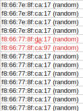
Image Description: We can see from the collected MAC address above, two of them are reported differently, although the human in us knows that it’s all the same.
Analyzing the example image above, we see that two of the collected MAC addresses are different from the general pool of MAC addresses. This same idea goes for ScanA addresses and Local Names. The outcome of this would be data congestion, tons, and tons of data that wouldn’t be useful at a larger scale. To break this further, if scanning a single device, the data representing that device will look like multiple devices, thus throwing the skew off later down.
Levenshtein Distance
Vladimir Levenshtein is a Russian mathematician who published this notion in 1966. I am using his distance measure to calculate the difference ratio between two strings. If two strings are higher than a certain percentage, it will consider them the same and replace the compared string with the higher value one.
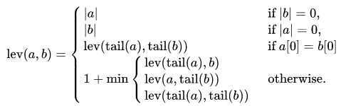
Image Description: The Levenshtein distance between two strings a,b.
Moving forward, we’re using a compiled package variant of ‘python-Levenshtein’ to do the calculations on the ratio of two strings or string to list value. The below code is a quick break-down of the algorithm that translates and formulate the balance.
	adva_list = df["AdvA"].tolist()
	strip_list = [item.strip() for item in adva_list]
	items = Counter(strip_list).keys()
	words_to_count = (word for word in strip_list if word[:1])
	ca = Counter(words_to_count)
	all_list = ca.most_common(len(items))

    l = []
	s = []
	for i in all_list:
		if i[1] > MC:
			l.append(i)
		else:
			s.append(i)
	l.reverse()

    rep = []
	new_l = []
	for i in l:
		a = process.extract(i[0], l, limit=2)
		if a[1][1] > PerR:
			top_current = (a[0][0][1])
			top_check = (a[1][0][1])
			if top_current <= top_check:
				chge = ("{}*{}".format(a[0][0][0],a[1][0][0]))
				rep.append(chge)
				new_l.append(a[1][0])
			else:
				new_l.append(a[0][0])
		else:
			new_l.append(a[0][0])
To expand further, we have a list of all MAC addresses within the AdvA column. This column is pipped into a list, stripped, and then counted. So we’ll have a list that now has the MAC address in its first part, and the second part is how many times that MAC address appeared in the list.
[ MAC, <# of time it appeared in list> ],[f8:66:77:7e:8f:ca:17, 130]
From here, it’s broken down into two separate lists, one being l (L for long) and the other being s (S for short). This is done by checking against MC (Match Count) variable. This variable is dynamically set in the upper end of this script file. Version 2 of these modules will utilize Machine Learning from Tensor-flow to calculate the best optimal value for MC. Nevertheless, if the second portion (# of time it appeared in the list) is more than MC, it’s pipped into the L list, and if it’s less, it’s pipped into the S list.
From there, we’re looping through the L list and first making a comparison against all MACs that might be a slight duplicate from itself. If the LD ratio is more than PerR (Per Ratio), it will continue the process. Since there is a hierarchy system between MAC addresses, it will use whichever MAC addresses have more values in the list and change the one below that to itself. This is then pipped into a new list, which the process is repeated against the S list. Version 2 will have a loop count based on a certain threshold to repeat, looking for similar patterns.
All values within the three main MAC address fields (AdvA, InitA, ScanA) are grouped and replaced together, and output to a new column is appending ML to its name. In short, if a value that was original found within the AdvA column is added to the replace list, if that value is anywhere in the two other fields (InitA & ScanA), they will be replaced and introduced in the new ML column.
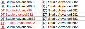
Image Description: Example of the Left side being the initially collected information, and the right side shows it after the machine learning aspect. (Highlighted in red is the changed values)
From my testing, we notice a reduction in noise values at 80%. This all adds to the bigger picture down the line when we plot these values against a graph.
Script
Machine-Learning.py will be second script to run. This script takes two arguments, input and output.
python3.8 Machine-Learning.py output.csv ml-output.csv
This script will create four additional columns:
- Local_Name_ML
- AdvA_ML
- InitA_ML
- ScanA_ML
With processing 1 million packets capture and with a regular Ubuntu workstation, it took less than 30 seconds to process the output.
Mac-Changer.py ::
Background
MAC stands for Media Access Control. You can think of it as a unique identifier for an electronic device connecting to a network, like a VIN for a car on a freeway of other vehicles. A Bluetooth address, sometimes introduced to as a Bluetooth MAC address, is a 48-bit value that uniquely distinguishes a Bluetooth device. There are two main types of Bluetooth addresses: Public & Random.
Bluetooth’s public address is a constant worldwide address. It never changes and is registered with IEEE. It endures by the same guidelines as MAC Addresses and is an extended unique identifier EUI-48. Random addresses do not need any registration with the IEEE. It is an identifier that is either programmed within the device or created during runtime based on the subtype.
Mac-Changer.py is used to associate an alphanumeric string to something that is finger-printable. This script utilizes the database of all registered IEEE Mac addresses, that’s free to download from:
https://macaddress.io
Essentially, the first three octets of a MAC address is what we do our comparisons against it. At the code level:
def check(search_string):
    with open('macaddress.io-db.csv', 'r') as f:
        csvReader = csv.reader(f, delimiter=',')
        for row in csvReader:
            MAC = str(row[0])
            CompanyName = str(row[2])
            if search_string in MAC:
                return CompanyName[0:8].strip()
        return False
if any([substring in InitA_ml for substring in matches]):
    search_string = InitA_ml[0:8].strip().upper()
    last_bit = InitA_ml[8:]
    line = check(search_string)
    if check(search_string):
        InitA_ml = line.strip()+last_bit
We’re first only doing this check against MAC addresses that are public. Random addresses wouldn’t have an association with IEEE. From there, we’re spiting the first three octets and running that against the check function, which will see for any matches. If there is a match, the CompanyName parameter is returned and used to replace the first three octets with the company name’s first eight characters. This process is repeated for all fields with mac addresses and all ML fields with mac addresses: AdvA, InitA, ScanA, Adva_ML, InitA_ML, ScanA_ML.
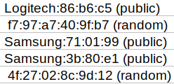
Image Description: We can see that Logitech and Samsung replaced the alpha-numeric characters.
Script
Mac-Changer.py will be third script to run. This script takes two arguments, input and output.
python3.8 Mac-Changer.py ml-output.csv mac-ml-output.csv
With processing 1 million packets capture and with a regular Ubuntu workstation, it took less than 20 minutes to process the output.
Graphs.py ::
Background
Network diagrams (also called Graphs) show interconnections between a set of entities. Each entity is represented by a Node (or vertice). Connections between nodes are represented through links (or edges). The graph is a force directed by assigning a weight (force) from the node edges, and the other interconnected nodes get assigned a weighted factor.
BTLE packets will always have the AdvA (Advertising Address) field filed out. This can be considered the Node, and any other listed MAC address listed will be viewed as the edge.
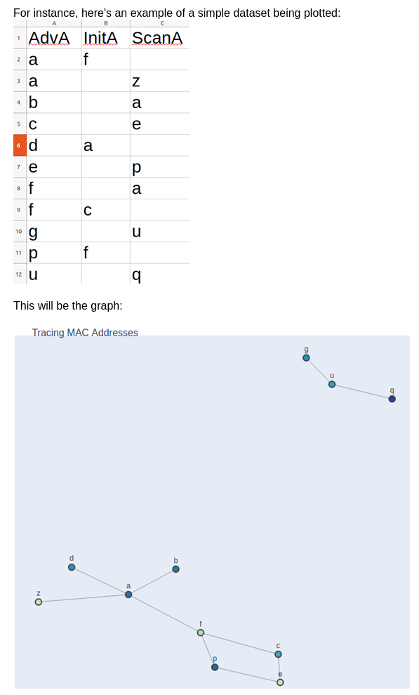
Image Description: We can see how each point is interconnected with the sample CSV data above in a very aesthetically pleasing way. G - U - Q shows that they all correlate together but don’t have any associated with any other points. (This particular graph doesn’t show directional or weight, just an example graph)
This script prints out two separate files, the edges and nodes.
Edges
The Edges are outputting the following information: TransactionAmt, Source, Target.
TransactionAmt is the number of times that that particular Source and Target pair have packets.
157, 86:2a:fd:42:f2:ee (public), 68:6a:e8:2d:93:b4 (random)
In this example, the MAC 86:2A and 68:6A have 157 different packets with each other. This value 157 is the weight value used in the next script to determine the line thickness (network traffic) between two devices.
Nodes
The Nodes are output necessary foundational information. Circling back to the beginning with the original collection: RSSI, PDU Type, Manufacturer are all part of the original packet. Essentially, this portion is going through all .
> 86:2a:fd:42:f2:ee (public), -87, SCAN_REQ:456, ADV_DIRECT_IND:3, Manufacturer Name
> 68:6a:e8:2d:93:b4 (random), -87.0, SCAN_REQ:4479, ADV_DIRECT_IND:11, Apple. Inc.
A few things are going on here. First, it’s taking the MAC address and going through the overall CSV document to find all MAC associations and all RSSI values. It will follow up and calculate the Median value for RSSI. In this example, it’s -87.
The second portion is doing the same, going through the document where that MAC address had any association with various PDU_Types, calculating and giving you the # of times it called that PDU packet. In the example above, the SCAN_REQ PDU type was sent 456 times from the first MAC address.
The Last part lists all associated Manufacturer that was collected; it will group them all and print it in one statement (duplicates removed).
Script
Graphs.py will be fourth script to run. This script takes one arguments, input.
python3.8 Graphys.py
With processing 1 million packets capture and with a regular Ubuntu workstation, it took less than 15 minutes to process the output.
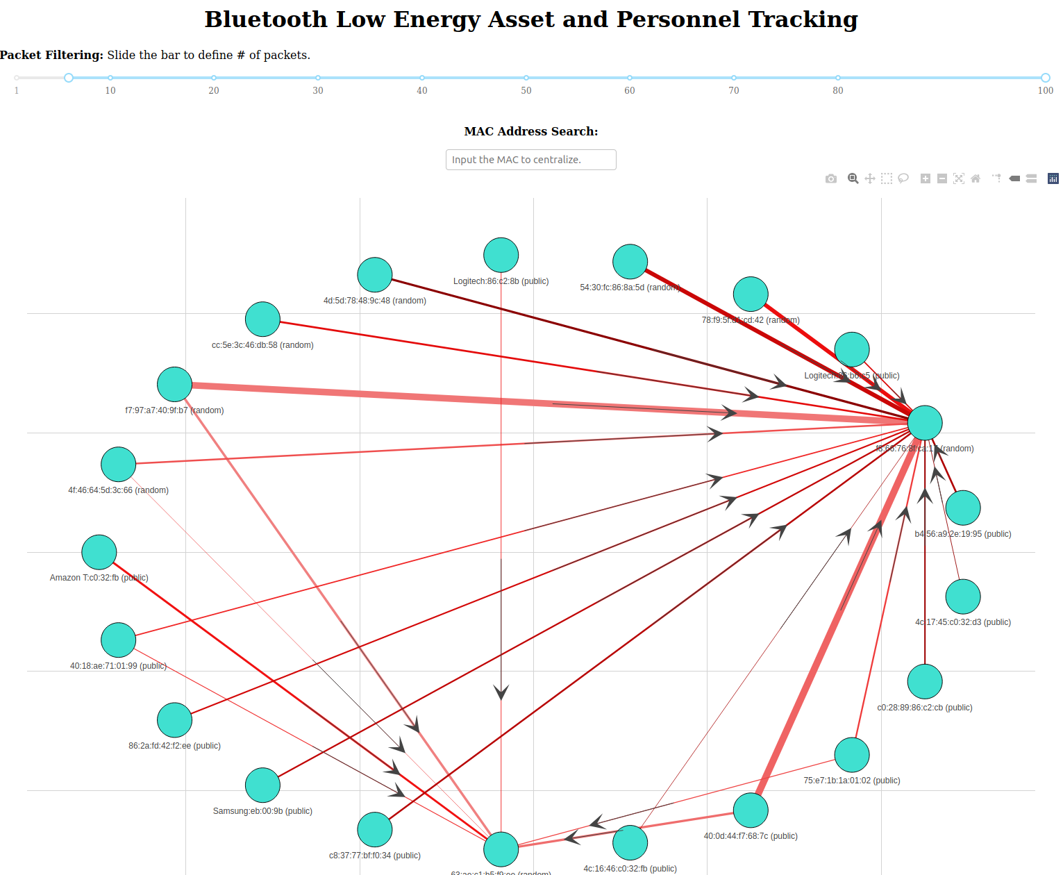
Web.py ::
Background
With the newly created Edges & Nodes file, Web.py utilizing both of these files to spin up a web-server and make an interactive Python network visualization app using NetworkX, Plotly, Dash.
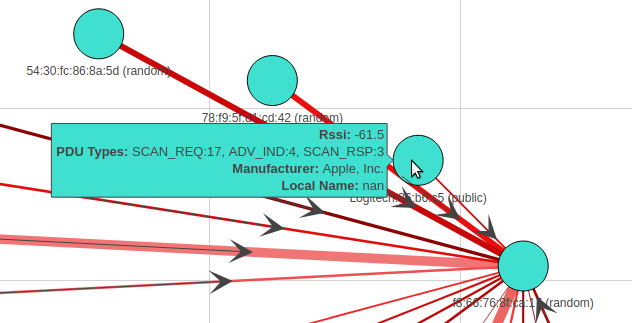
This would make a directional graph, meaning the arrows will point to which traffic is flowing. The next bit is the line thickness is determined by the weight value, which is the number of packets per that conversation.
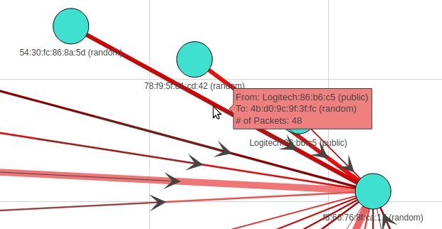
The last bit would be when you highlight a Mac Address, and it will give you all the attributes for that address!
Script
Web.py will be the last script to run. This script takes no arguments. Both graph-Edges.csv & graph-Nodes.csv would need to be in the same directory as Web.py
python3.8 Web.py
The web server has two excellent filters, MAC address search, and Packet Filtering. Mac Address Search will center whichever packet that is being searched. Packet Filtering sets the threshold for what kinds of packets to show; in this case, it’s anything more than five packets. If set to 1, the graph might not be readable as it will showcase every packet. In this case, 1 million will be showcased and might crash our system. Packet filtering defaults at five or more packets (transactions), and it will be displayed.